Newsletter Article

Reporting Options in SA -- Controlling Vectors

Taking measurements in metrology is half the battle—the other half is reporting your results in an understandable and meaningful way.  Producing a 2D printable report that fully illustrates a complex 3D evaluation of an object can be a significant hurdle; however, recently added advanced reporting tools in SpatialAnalyzer (SA) can help.  Vectors provide a means of visualizing small distances and the tools to capture 3D objects in clearly-illustrated 2D images.  Learning to manipulate the visual display of vectors can greatly improve your ability to illustrate your work.   Read on for more about controlling vectors in SA.

Taking measurements in metrology is half the battle—the other half is reporting your results in an understandable and meaningful way.  Producing a 2D printable report that fully illustrates a complex 3D evaluation of an object can be a significant hurdle; however, recently added advanced reporting tools in SpatialAnalyzer (SA) can help. 

Vectors provide a means of visualizing small distances and the tools to capture 3D objects in clearly-illustrated 2D images.  Learning to manipulate the visual display of vectors can greatly improve your ability to illustrate your work.   Read on for more about controlling vectors in SA.

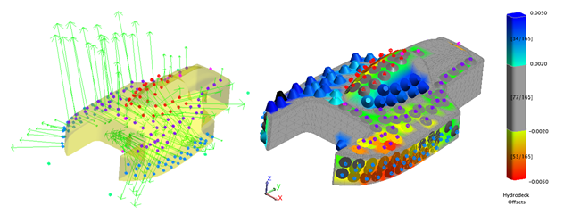
Above: Vector group display prior to editing (Left), and after editing (Right)

Creating Vectors

There are two fundamental approaches to building vectors:

1. 1. Queries

2. 2. Relationships

The settings and controls for vectors are the same regardless of whether they are built from a relationship or query. 

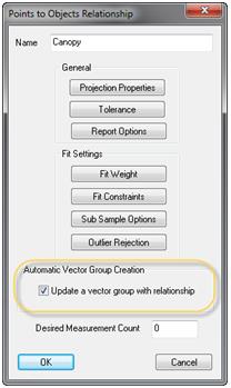
The first step in creating vectors is to decide whether you want to capture a snapshot in time or build a dynamic indication of point-to-object deviation.  Like anything in SA, a vector group created by a query is a static snapshot unless it is tied to an object through a relationship.  Therefore, if you want the vectors to update and continue to display the current orientation of the points and objects, use Relationships.  To build a dynamic vector group, simply build a relationship between your points and objects, and then go to the properties of the relationship. There you will find an option to turn on an Automatic Vector Group, control its projection options, and set its tolerances.  If at any time you wish to convert an auto-vector group into a static vector group, just go to the properties of the relationship and turn off the update option.   Doing so will not delete the vector group, but simply leave it as a snapshot that can be used later for reporting or review of alternative alignments.  You can also right-click a relationship and select “Make Vector Group (static).”

Projection Options

When you build vectors, there are some initial decisions to make.  The first step is to decide how you want to display probe offsets.  SA automatically accounts for the probing offset, so the distance between the measured point and the measured surface is equal to the probe radius.  In order to properly compensate for the probe offsets, SA calculates the distance from the measured point to the surface and then subtracts the probe radius from that distance.  This provides the user with the exact position of the contact point between the probe and the surface (for more detail, see the section on Probe Offsets and Surface Normal Direction in the SA User’s Manual).  This measured position can then be compared to a nominal or design position. 

Vectors can be drawn in four different ways, depending on the way in which you wish to represent the start and end condition of the vector and the way in which you want to display the probing offset.

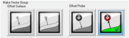
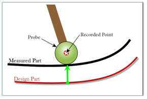
By default, SA uses a vector display scheme that draws the vector lines from the closest point on the part’s surface to the contact point on the probe.  This inspection approach provides an easy way to display the relative deviations in the size and shape of a measured part as compared to a nominal part.  Alternatively, the vector lines can be drawn in the other direction to display the relative probe position compared to the surface, which provides a build perspective rather than an inspection.

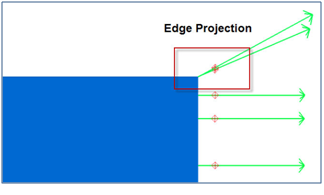
You must also decide if you want to include Edge Projections.  Vectors will show the straight line distance from an object to a point regardless of whether the point is on the surface or offset beyond the edge of the surface.  In such cases, these points can have a significant impact on the average and maximum vector deviations reported for the vector group, but leaving them on can be very helpful for visualizing misalignment between parts.

Vector Properties

The vector properties dialog can be accessed by double-clicking on any vector group.  Within the properties you will find three primary elements:

1. 1. Basic statistics summary

2. 2. Display options

3. 3. Tolerances

The default settings for any new vector group can be edited by going to the User’s Options>Display Tab>Colorized Object Options.

Display Options

The controls for the vector display are divided into two sections:  the representation method and the scale.

Deviations between measurements of a part and the design part in metrology are typically quite small, on the order of hundredths or thousandths of an inch.  For the purposes of visualizing these deviations, vectors are drawn at 100:1 scale.  Therefore, if you have a one hundredth of an inch deviation in the part, the vector arrow will be drawn one inch long.  This makes it easy to see relative deviations that would otherwise be nearly invisible; however, this value can be easily adjusted in order to more effectively display relative distances.  The width of the arrow can also be adjusted.

Blotches are an alternative way of drawing a vector.  Blotches provide a colorized indication of the relative vector length deviation, while tubes use the blotch size at the base and the vector length.  Using arrows, blotches, tubes, or a combination allows you to clearly illustrate the deviation between a single point and a surface, or create an exaggerated 3D view of the surface and its deviations.

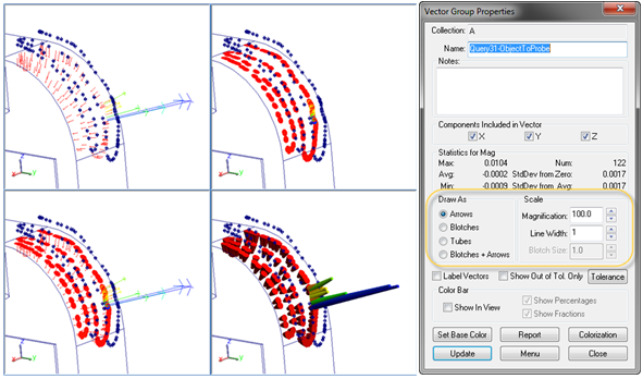
Above: Vector Line Display Options (Arrows, Blotches, Arrows + Blotches, and Tubes)

Tolerances and Colorization

Tolerances are either driven from a relationship or can be set in the properties dialog of the vector group.  It is important to point out that the tolerances set in these two places are different.  The tolerance for a relationship can be set for any vector component in addition to the magnitude, each of which can be evaluated independently.  To visualize the individual components of a magnitude vector, you can right-click on it and create the individual vector components as separate vector groups. A vector group; however, is only one component of this.  It can be set to show X, Y, Z, or magnitude independently, but can only show that one component for visualization purposes.  So, the tolerance set for that vector group is only a magnitude tolerance.

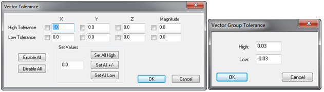
Above: Relationship Vector Tolerance Settings (Left) and Vector Group Tolerance Settings (Right)

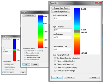Within the properties, tolerances can be set either with the tolerance button or by going to the Colorization options within the vector group properties and defining a tolerance region for colorization. Within the colorization options you have several choices regarding color range limits.  One of the more complex and informative options is the “Tolerance (Continuous)” option, which allows you to set the colors to display based on the range of out-of-tolerance vectors only. 

Any vectors within tolerance are displayed as grey by default and can also be hidden. Vectors that are below tolerance are displayed in a continuous range of hot colors, while vectors above tolerance are displayed in a range of cold colors (this base color choice can also be changed with the base color button).

Above: Colorization Schemes (Toleranced (Go/No-Go), Continuous (Entire Range), & Toleranced (Continuous)

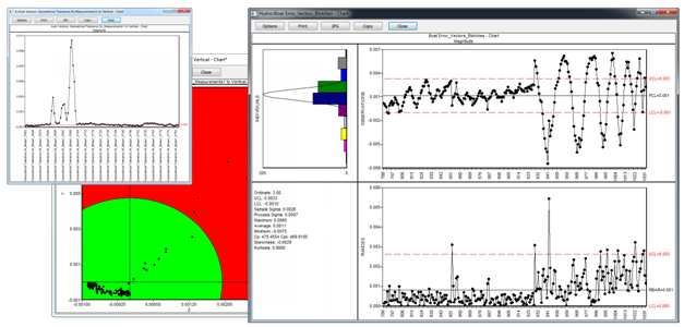
Once your vector group has been formatted to your preference, you can capture a screen shot of the vector group from any view point by using the camera icon.  From there, you can drag and drop the image into a report.  Alternatively, you can right-click on a vector group and generate a quick report, which will capture the current graphic image and place both the image and the vector group report table in a new SA report.  More traditional standard 2D run charts and bullseye charts are also only a right-click away.

Building a Report

A simple vector report can be obtained directly through the vector properties dialog, but you can access more reporting options by adding a vector group to an SA Report.  Dragging and dropping either a relationship or a vector group into an SA report will generate two tables:  a summary table with the basic statistical information and a details table showing the individual vectors.  The individual reporting options for any object are saved with that object and operate

independently unless you apply the settings to all.  These settings can be accessed either by right-clicking on the vector group in the tree and selecting Reporting Options, or by right clicking on the table directly in the SA report.  Important reporting options to consider for a vector group are as follows:

1. 1. The Reporting Frame

2. 2. The Coordinate System (Cartesian, Cylindrical, or Spherical)

3. 3. Components to Include

4. 4. Report Format

One of the most important things to keep in mind when reporting your results is that current position and orientation of any object is reported relative to the active coordinate frame, unless you specify otherwise.  SA reports are dynamic, so the reporting frame for all objects in the table will update if you change the active frame.  So, if you wish to report the locations of objects relative to a different coordinate system it is important to set that specific frame as the reporting frame, a setting that can also be accessed by right-clicking.

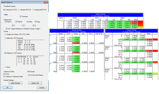
Shown Above: Reporting options dialog and optional report formats available to SA users

Example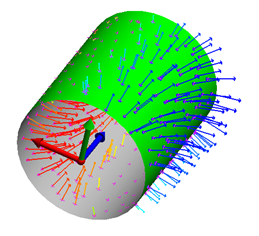

As an example, let’s consider a case where you want to report point deviations relative to a central axis of a cylindrical part while continuing to report the rest of the job based on a different primary coordinate system.  To view your point deviations relative to this central axis, you can set your coordinate system to “Cylindric (R/T/Z),” which will allow you to report deviations as radial from the central axis, vertical high (z) from the centroid of the frame, and theta (horizontal angle, theta).  In order for this coordinate representation to make sense, you would set the reporting frame to be a frame on the central axis of the part.  This would provide an immediate display of the concentricity of your part at any point relative to the central axis.

Questions? Do you have any hints or tips of your own that you’d like to share? Contact NRK at support@kinematics.com.

Sign up to receive our eNewsletter and other product updates by clicking here.